Higher Importance
Medium Importance
Lower Importance
–
Preface

Exocoetidae is a Family of fish that looks that it has wings and appears to fly over the surface of the water. These characteristics have led to this fish being commonly referred to as “Flying Fish.” However, they do not actually fly; they glide. According to National Geographic, “their streamlined torpedo shape helps them gather enough underwater speed to break the surface, and their large wing-like pectoral fins get them airborne.” They swim downwards with great speed, up to 37 miles per hour, and then angle upward towards the surface of the water. Using this momentum, the fish is able to break the surface of the water with enough force to propel itself into the air and then uses its fins to glide. After some time in the air, the fish will return to the water. Depending on the speed, energy, and size of the fish, the height and length of the glide can vary. But what does this have to do with the NFL? More than you might think.
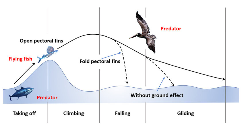
In terms of physics, there are natural forces in action on both sides of the surface of water. The Flying Fish uses the buoyancy force (and upward momentum) below of the surface of the water in order to counteract the downward force of gravity when it is later above the surface of the water. The NFL has rules that create a macroeconomic environment that is similar to the natural environment within which the Flying Fish lives. These rules will be further explained below, but in general, the league pushes organizations toward an equilibrium of a 0.500 record (an equivalent number of wins and losses), just like buoyancy and gravity push objects toward the surface of the water. The goal of the Flying Fish and an NFL organization is the same: to glide above the equilibrium. For the Flying Fish, the glide above the surface of the water is for escaping underwater predators; for NFL organizations, the glide above the equilibrium is for making the postseason. How an organization operates within the NFL will determine the height and length of its glide (or, in other words, its “championship window”). Scientists are able to observe and measure the actions of the Flying Fish, but what about the path of NFL organizations? The foundation of this project is to plot and measure the path of NFL organizations in a more detailed, and ideally more accurate, way other than just the number of wins in a season. Hypothetically, if one could create an accurate model to evaluate the actions of an NFL organization, then he or she could accurately predict its path or, in other words, its future performance.
–
Introduction
Everything in life revolves around cycles. Life itself is a cycle. In humans, the blood in your veins, the oxygen in your lungs, the saliva in your mouth: all part of a cycle. In nature, the water in a river, the seed of a plant, the position of the sun: all part of a cycle. Even in machines that humans have created, pressing a gas pedal, turning on a light, charging a phone: all part of a cycle. While a circle is typically used to represent cycles, as the shape is formed by a constant, uniform movement that ends where it begins, a waveform is another way to show a cycle. The waveform allows the opportunity to more easily express the elements of a cycle with respect to time. For example, light and sound are cycles. Despite being invisible to the naked eye, these cycles are translated by eyes and ears to create images and sounds. Light and sound are typically graphed as a waveform, therefore including the element of time, which has allowed scientists to map and measure them more easily. The frequency, wavelength, and amplitude of light and sound waves will determine what one sees and hears. The scientific method implemented to make those discoveries is also a cycle.
Even an economy is a cycle. Should sports be any different? At many levels, they are not. The tennis shot is a cycle. The act of running is a cycle. Taking a step back, let’s look at the cycle of sports at a higher aggregation. Alternating who serves the ball and which side of the court each player occupies in tennis is a cycle. Track is running around a circuit. While the long-term performance of the athletes in these individual sports can be cyclical (training to get better during the early stage of their career, peaking during their athletic prime, and then fading in performance as they age out of their prime years), athletes typically retire before they drastically decrease in performance, therefore hiding the return toward the beginning of their respective cycles. However, that is not the case within team-based sports leagues. The cycle of performance can be easier to see than the cycle of the individual athlete, because the organization’s downfall in performance can’t be hidden by retirement. An NFL player can retire, but an NFL organization cannot. The clarity of cycle depends on the economic environment of the individual league. The structural rules of the league, such as salary limitations and scheduling of opponents, will determine the cycles. For example, the cycles of English Premier League are difficult to see. One could argue that there aren’t any cycles at all but rather just small, random movements. While there are theoretically some salary limitations to control how much money a club can spend on its players, the top clubs are still allowed to outspend the smaller ones. And because the top-performing Premier League clubs earn automatic bids to play soccer in the Europe-wide competitions (Champions League and Europa League), which pay out large sums for participation, larger clubs with more financial resources are incentivized to spend large amounts on high-end talent from around the world. The largest English clubs are known as the “Big 6” (Manchester United, Chelsea, Liverpool, Manchester City, Arsenal, and Tottenham), but any club can attempt to join the ranks of the Big 6 if they have the funding. In 2021, Newcastle United was purchased by an investment group led by the Saudi Public Investment Fund (PIF). From 2020-2025, Newcastle had the 5th-highest net spend, spending more on players than both Manchester City and Liverpool. In the 2024-25 season, they finished 5th in the league, taking one of the 5 automatic bids to the Champions League for the following season. While these Big 6 clubs are not always in the top 6 positions in the league (especially shown by the 2024-25 season), they will always have an advantage over the smaller clubs. This advantage means that the performance in this league is not clearly cyclical. Bigger clubs do not need to undergo a period of lower performance in order to be better in the future, as there is no long-term incentive to perform worse, but instead there is always a long-term incentive to spend more in order to perform better.

The disincentivization to perform worse is sustained by the other economic movement of the Premier League: the relegation system. The three worst-performing Premier League clubs drop into the second-highest division in the English football league system (the Championship) for the following season, decreasing the money that they will receive to spend on talent. On the other hand, the three best-performing clubs of the Championship get promoted into the Premier League in the following season. This move gives the promoted club a large increase in money to spend on better talent in order to try to compete against the other Premier League clubs in the following season. The semblance of a cycle comes from the fact that there is a set of clubs that go through these two moves over and over again, switching between the two leagues, their resources constantly growing and contracting. Instead of English football organizations (clubs) being in any phase of a cycle, they are relatively static in one of these types: Big 6 (or ~8 largest clubs perennially competing for Champions League), Mid-Table (relatively safe from relegation, sometimes competing for Europa League/Europa Conference League), Relegation Zone (typically recently promoted clubs, attempting to do well enough to not get relegated). These designations are almost entirely determined by their level of resources and how much money an organization is willing to spend. Similar to the athlete, the historical movement of any individual club is not universally witnessed as many people only follow the Premier League or only watch the Champions League. The cycles in the Premier League are within the types but not across the entire league. The two main cycles (or, in other words, feedback loops) are at the top and the bottom of the league. At the top is the Champions League cycle: Phase 1 is spend a lot on players/facilities, Phase 2 is perform well enough to earn a bid to European competitions, and Phase 3 is to recycle that money to fund and improve the club (same as Phase 1). The longer a club is able to stay within this cycle, the larger the club. Falling out of this cycle can cause a club to shrink due to receiving less money by failing to qualify for the Champions League. At the bottom is the Relegation cycle: Phase 1 is to spend enough on talent to get promoted to the Premier League, Phase 2 is to perform well enough to stay up (avoid getting relegated), and Phase 3 is to recycle that money to improve the club in order to remain in the league (same as Phase 1). Falling out of this cycle can cause a club to get relegated and therefore shrink. The cycles of the Premier League, and most European football leagues, are not strictly performance-based but are instead financial cycles, which influence what size and, therefore, what type each club is.

The Premier League can be considered an open economic environment. Outside factors, such as the European competitions, influence the financial hierarchy, and the poorest-performing clubs can actually be removed from the league entirely (via relegation as mentioned earlier). American team-based leagues are closed, in that they do not have a Champions League nor a relegation system, so organizations are not affected by outside forces. This difference makes them more insularly cyclical with respect to the performances of the individual organizations. The least cyclical American team-based league is the NBA, which has a “soft cap” salary system. The soft cap means that an organization can spend over the set limit as long as it pays a financial penalty. This condition means that, to an extent, an organization can outspend others if the owner is willing to pay the “Luxury Tax.” The MLB also has a soft salary cap, but it is instead called the “Competitive Balance Tax,” which works similarly to the NBA’s luxury tax. If an owner is willing to pay extra, their organization can outspend the others. In these two leagues, worse current performance does not necessarily translate to better future performance if the competition can constantly spend more to have better talent. Additionally, the drafting process is an element that every major American team-based sport has that non-American team-based sports and their leagues typically do not have. The organizations of American professional sports are entitled to secure pipelines of young talent, whereas that does not exist in, for example, European soccer. In the MLB, NFL, and NHL, the draft order is determined strictly by the previous season’s performance of each organization in relation to each other. However, the NBA has a draft lottery, within which the worst-performing organizations from the previous regular season have the best chance to get the top pick of the eligible young talent that have declared for the draft. However, other than the worst team guaranteed to not have worse than the 5th pick, they are not guaranteed any pick position. The better an organization performs in any given season, the worse the chances of getting a better pick in the following draft. The 2025 draft lottery is an example of the draft lottery messing with the league’s cycles of performance. The 2024 Dallas Mavericks, who finished 19th out of the 30 teams with a 39-43 record, had a 1.8% chance of winning the #1 pick but were selected regardless. That means that the 10 worst organizations that really needed that pick in order to potentially add a future superstar will not be able to.
One could argue that the NFL is the most cyclical league in the world. It has a hard salary cap, meaning that no organization can consistently spend above a set limit, so it cannot simply outspend the others. Not only does this rule make the NFL typically more competitively balanced than other leagues, it also makes the roster decisions of an organization more influential to its performance. Inefficient talent management cannot be covered by spending more than other organizations like it can be in European football. As stated earlier, it does not have a draft lottery; the order of the NFL draft is instead determined strictly by the previous season’s performance of each organization in relation to each other. Unlike other leagues, NFL organizations do not play every other organization in the league. That irregularity may seem unfair, but the schedule is set up so that the better teams from the previous season have a harder schedule, and the worse teams have an easier schedule. Poorly-performing organizations will naturally be pushed to be better in the future, and well-performing organizations will naturally be pushed to be worse in the future. The cyclical nature of the NFL gives the league a reputation of being egalitarian, as neither the size of the organization’s home market nor wealth of the organization’s owner should determine success or failure. Elements like talent management off-the-field and time management on-the-field should be more influential to the organization’s performance. Mapping the cycles of performance of individual organizations over time creates waveform structures. The purpose of this project is study these waveforms over time in the same way that scientists studied the waveform structures of light and sound. If one could create a model to accurately access the cycle of performance of an organization, then one could track it over time and make accurate predictions of future performance.
–
The Economic Model
The IMF (International Monetary Fund) defines an “economic model” as “a simplified description of reality, designed to yield hypotheses about economic behavior that can be tested.” In this case, the reality is the set of actual Win/Loss records of the 32 organization that comprise the NFL. The hypotheses yielded are the predictions (not only the Win Total estimates, but also the predictions about Coach Scores, GM Scores, etc.). Economic behavior here is the set of measurements of performance outside of just wins and losses. The foundation of this project is figuring out how to create those measurements in order to evaluate NFL organizations other than number of wins or playoff appearances.
An NFL organization is comprised of two main groups (of non-players): the Front Office and Coaching Staff. The Front Office (lead by a General Manager – GM) is responsible for accumulating players (either through drafts or free agency), and the Coaching Staff (lead by a Head Coach – HC) is responsible for optimally leveraging those players in order to produce the highest possible level of on-the-field performance.
The GM Score measures the performance of the Front Office is two ways: Power and Efficiency. Power measures how much the organization is spending on its roster of players. Efficiency measures how accurately the organization is paying those players with respect to performance. Efficiency is then broken down into Balance and Talent. Balance is how efficiently the organization is paying the various position groups (QBs, RBs, etc.) with respect to the performance of the team overall. Talent is how efficiently the organization is paying the players individually with respect to the performance of the individual players. Performance at the player level is evaluated by the Approximate Value metric developed by Pro Football Reference, and the salaries and salary cap information are provided by Spotrac.
The Coach Score measures the performance of the Coaching Staff in several ways. While the number of wins are typically considered what matters the most, there are different ways to ways to assess a win. Factors like one-possession wins (wins by a margin of 8 or fewer points) or consecutive wins in a row are rewarded, while close losses and consecutive losses are penalized.
How a Coaching Staff utilizes the cards that they were dealt by the Front Office determines whether or not they are able to win the hand. Ideally, these two groups are working together in order to run the best organization as possible. This relationship is vital as their fates tend to be intertwined. The GM Score and the Coach Score are combined, creating in the ORG Score, which is the measurement of the overall performance of the organization. ORG Score is then converted to Win Total predictions (ego).
All of the Scores for each NFL organization from 2015 to present can be found here. Predicted Scores begin in 2020.
–
Hypothesis – Cycle of Performance
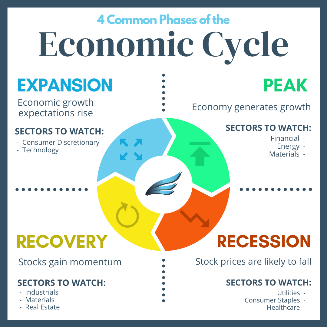
As mentioned in the Introduction section, there are a few rules that are unique to the NFL which give the league an economic environment unlike the other professional leagues in the US and around the world. Primarily for this project, the hard salary cap, draft order, and schedules are the main guardrails that guide the competitive balance of the league.
The hard salary cap means that organizations cannot simply just outspend the other organizations in order to achieve a higher performance. Every organization must spend within the range of the salary cap (including the minimum limit). The salary cap rolls over, meaning that a portion of the amount that an organization does not spend of the salary cap in any given season rolls over into the next season’s “budget.” Therefore, an organization could forgo current spending for future spending, with the hope that the extra budget that has rolled over will result in higher future performance.
The draft order is determined by the previous season’s number of wins (including the playoffs). The organizations will draft new players in the ascending order of wins, with the organization with the fewest number of wins drafting first and the one with the highest number of wins drafting last. This rule theoretically encourages organizations who know that they are not going to perform well enough to make the playoffs to intentionally lose games in order to increase the value of their draft position. This controversial practice is know as “tanking.” A common argument against the existence of tanking is that players would never intentionally play worse in order to benefit the organization long-term. I completely agree. Just making the NFL is incredibly difficult, and no one would risk that for an organization to be better in future seasons when that player may not even be on those rosters. However, that it not what tanking is. Tanking happens at the organizational level. The players are certainly trying their hardest to have their best performances on the field, but the tanking Front Office has intentionally put together a roster of players who just simply are not as good as others on the rosters of other organizations, no matter how hard they are trying.
The schedule is also designed to level the playing field across the league. Teams are scheduled to play their fellow division members twice a season, and then another set of matchups are determined by random. However, there is a third set of matchups for each team that is determined by the previous season’s results. 1st place teams from the previous season will play other 1st place teams, 2nd place team will play other 2nd place teams, etc. This practice allows for the NFL to guarantee quality matchups so that they can therefore guarantee high TV viewership. However, that also means that the worst teams from the previous season will be scheduled to play each other. While that give formerly poor teams a better chance to have more wins in the latter season, it can also make for some underwhelming football at times. I should note that the NFL is tied with the NHL for the American league with the most teams (32 – the NBA and MLB have 30). So while some games between two organizations that performed poorly last season might not be the most exciting, but with 13-16 games per week, there should be at least 10 quality games a week. The Premier League, for comparison, has 20 clubs, so at best it has 10 quality matches per week.
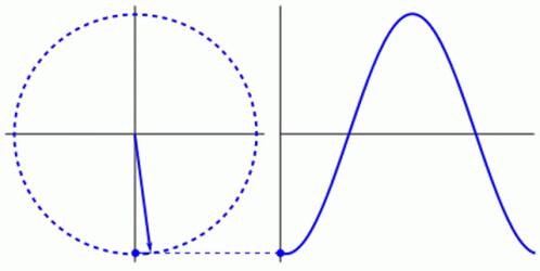
Through these three rules, organizations are pushed toward a 0.500 record (equivalent number of wins as losses), in that good teams from the previous season are given a tougher experience in the following season, while bad teams are given a step up. If one assumes that the goal of an organization is to have the best team possible (resulting in the best opportunity for a Super Bowl win), then what are the actions required to do so? Organizations have learned to adapt their behavior to these regulations by intentionally pushing the performance of the team either up or down. It is a similar situation to being asked to jump as high as possible. Almost every single person would bend their knees, lower their center of mass, and then use their legs to propel themselves upward. If 0.500 is a person standing still and upright, then that person would need to go below 0.500 in order to propel themselves above 0.500. If that same person were asked to keep jumping, then they would likely use the downward momentum of the previous jump to efficiently lower themselves into the first sequence of the next jump. If one plotted the person’s Vertical Location as the Y-axis and Time as the X-axis, the function would be a waveform. Additionally, the lower the person lowers themselves (to a point), the higher that they can then potentially jump.
As time goes on, the performances of the individual NFL organizations become cyclical as well. Let’s visualize the cycle with a graph.
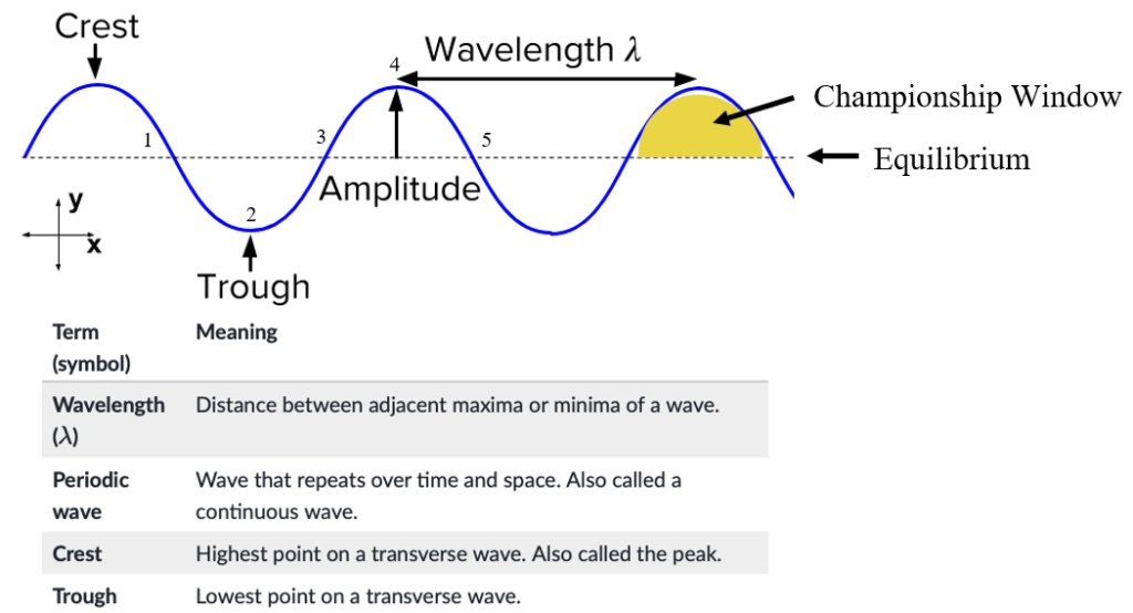


In order to more granularly translate the jumping motion into the performance of an NFL organization, let’s start at the same point. On this graph, that is at Phase 1, which is on the Equilibrium line. For the jumping analogy, Phase 1 was standing upright. For organizations, it is a 0.500 record (8-8-1 for a 17 game season). We are going to assume that the organization is also at the Equilibrium in terms of salary cap and draft positioning (number of picks and order). Here Equilibrium for salary cap means having used an average percentage of your salary cap, and Equilibrium for draft positioning means having neither traded away nor accumulated draft picks and being at the midpoint of the drafting order. An organization can start the cycle by making its roster as bad as possible by “pulling back” (also called “tanking,” will discuss later but basically trade any good players in exchange for future draft picks and spend as little as possible). This organization would then perform poorly (Phase 2), thereby earning better draft picks (for at least the ones that are naturally theirs, as the positions of the picks gained from the trades depend on the performance of the other organization involved in the trade), which can be used to build the foundation for potentially much better teams in the near future. If these new-drafted players play well enough (Phase 3), then the GM can use the rollover cap space that was gained from underspending in previous seasons to gain higher quality talent in the form of Free Agents. Ideally, this roster becomes much better than the Phase 1 roster, and, while the length may vary, this process of rebuilding up to this point typically takes around 2 to 3 seasons to accomplish. Depending on contract lengths, acquisition quality, along with other elements, the organization could have a couple seasons at Phase 4 (“peak seasons”) to compete for a playoff run with the hope of winning a Super Bowl. In these seasons, the organization will often be supplemented by Free Agency acquisitions from other organizations in exchange for future draft picks (what I call “pushing,” inverse of pulling back/tanking). This move is obviously risky as spending more now means that there will be little to no rollover in subsequent seasons, and there will be worse access to the newest labor pool (worse draft positioning), typically making future rosters worse. As contracts for top players reach the end of their lifespans, the organization will begin to not be able to pay all of its stars, as some of them will require large extensions to match their recent contributions to these high-performance rosters. After shedding some of the expensive star players over a couple seasons, the organization will return to its original state of having an average roster with some stars but mostly average to below-average players (Phase 5).
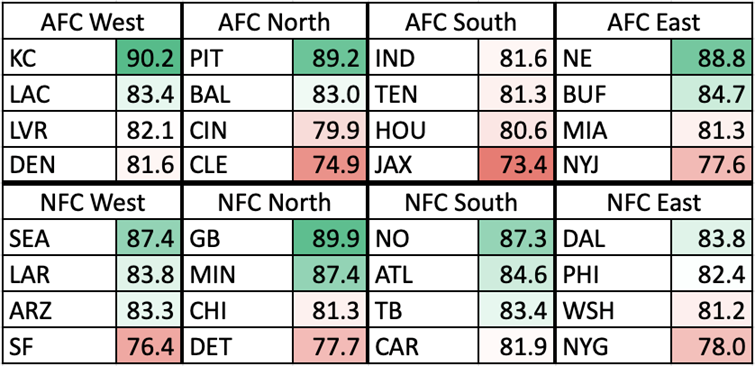
The cyclical process laid out above can vary in Equilibrium, Wavelength, and Amplitude depending on the quality of moves that the organization makes off of the field (along with the performances on the field). An organization that has a better Coaching Staff and Front Office, drafting quality talent and making sound Free Agency acquisitions, will have a higher Equilibrium. On the other hand, an organization with a worse Coaching Staff and Front Office will have a lower Equilibrium, indicating poor performance and roster management. Additionally, it’s important to know that these Organization Scores are in relation to the other organizations in the league, in that, they are all scaled to average around 82. All of the metrics used in this project are intentionally designed to match a generic American school grading system, hopefully making them easier to interpret. Theoretically, the Equilibriums of the Scores for all of the NFL organizations should be equal over a long enough amount of time. In the short term, there may be some variation, but as more and more seasons get added, the range of Equilibriums across the league should shrink. However, this theory would only hold true if every team were equally efficient with their assets, both current players and future draft picks. As this theoretical equality is not the case, the level of the Equilibrium will depend on the organization’s average asset management. Below are the Organization Score Equilibriums for every organization from 2015-2021:
–
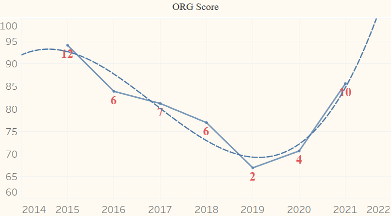
Below is a graph of the Organization Scores for the Cincinnati Bengals, one of the clearer cycles from 2015 to 2021. Unlike the example waveform in the labeled image above, this organization begins at a local Crest instead of the Equilibrium. The Score downfall from the Crest (2015) to the Trough (2019) is relatively smooth, much more than that of the Win Totals (indicated by the label at each point). For example, if one went by just number of wins, then 2016 would be below 2017. Essentially, Win Total is often not an accurate, encompassing representation of an organization’s performance. QB Joe Burrow was injured during the 2020 season, likely dropping the GM Score lower than it would have been. The curve would be much smoother if that injury had not happened (assuming that the Score would have been in the low 70s). The ORG Score Equilibrium for the Bengals over this period is slightly below average, at around 80, but thanks to the cyclical nature of organizations’ performances in the NFL, they had a wide range of performances. 2015 and 2021 were great seasons for the Bengals, bookending a death and rebirth of the organization.
Graphs for all of the NFL organizations can be found here.
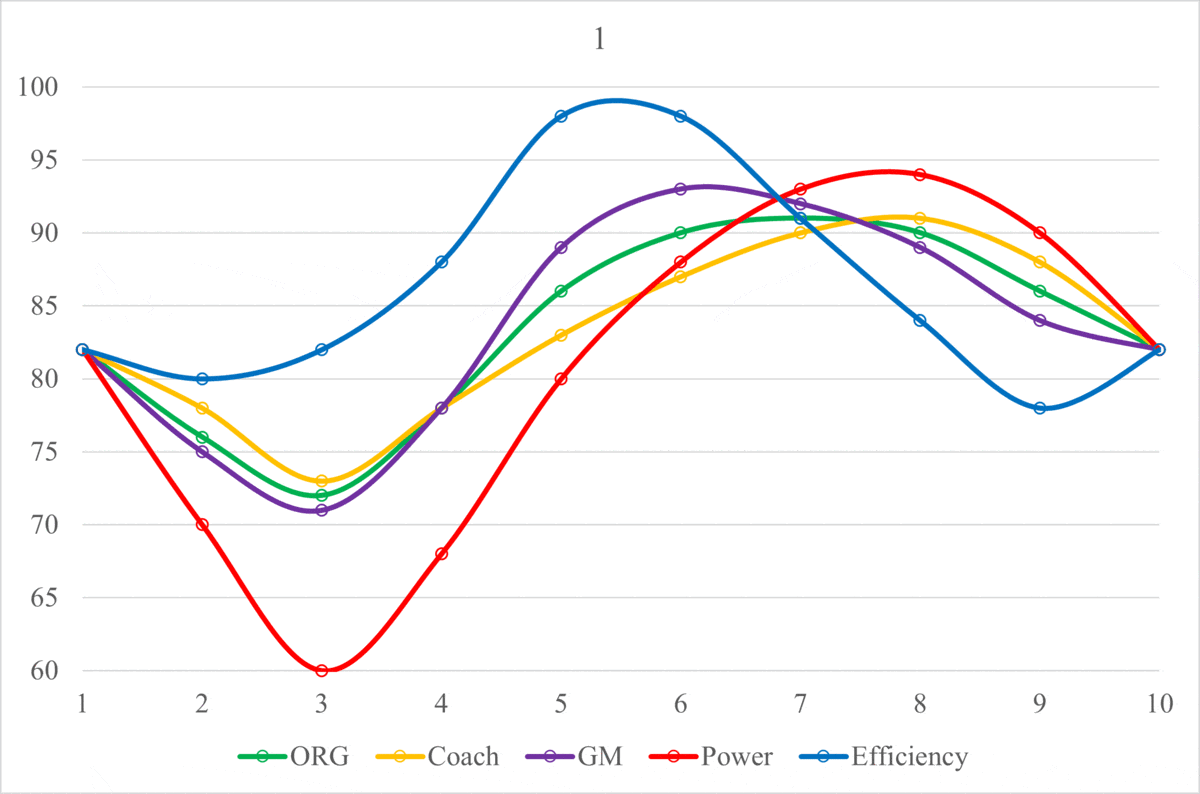
As this project is fed more seasons, the cycles should become clearer. The length of a cycle will vary based on the elements mentioned above, but 10 years should, on average, illustrate some cyclical qualities. Below is a generic example of the cyclical process shown in the gif above with the same exact metrics separated out but with the x-axis of time remaining static in this one. I should note that average of all of the metrics in the cycle below, as with the cycle gif above, matches the league-average of ~83 (except Wins, which is 8.5). While the colors attempt to singularly represent a much more complex set of decisions, they can, at the very least, help to show the general direction of the organization.
Red = entering rebuild / Blue = exiting rebuild / Green = front half of championship window / Yellow = second half of championship window
Red = pressing the brakes / Blue = putting the car in low gear / Green = putting the car in high gear / Yellow = taking the car out of gear but not using the brake
Here is another example of an organization that executed a rebuild into a championship window: the Buffalo Bills from 2015 to 2024. Compare the Bills chart below with the example from above. Organizations are rarely going to be able to exactly match a hypothetical “optimal” rebuild-window model, but this one is pretty close.
The Bills started in a yellow period, just coasting in “No Man’s Land” (not good enough to make the playoffs yet also not bad enough to generate valuable draft capital). From 2015 to 2016, they were stagnant in terms of their spending while remaining at an average level. Both the Head Coach and the General Manager were fired during or after the season (HC Rex Ryan the former and GM Doug Whaley the latter). The new GM, Brandon Beane, immediately (and correctly) turned the roster over, dropping the Power via eating the Dead Cap charges, which also decreased the Efficiency. The downward aspect of the rebuild (in red) continued into 2018, but the Efficiency increased, as they drafted a new, first-round Quarterback, who was therefore on a rookie (and therefore cheap) deal. Then the Bills entered the upward aspect of the rebuild (in blue) where they started building around their young QB with potential. They were able to open a championship window in just one blue season, when it could take one or even two more, thanks to the effectiveness of the Bills QB/HC/GM combination. Once the championship window was opened, there were two clear peak seasons in green (2020 and 2021). The Bills were able to increase both their Power and Efficiency in consecutive seasons while in a championship window, which is rare. However, there was a dip in Power and Efficiency in 2022, and while they did win 13 games (and therefore had a peak season), one could say that it was a step back in terms of roster. The Coaching Staff covered the decrease in talent well (Head Coach McDermott won the Sporting News Coach of the Year Award in 2022). 2023 was also somewhat of a stagnant season, as the window began to close. The Bills increased the Power, but it caused the Efficiency to decrease, creating a Power/Efficiency flip, where the Power becomes higher than the Efficiency. This phenomenon is typically an omen of an approaching rebuild, as the organization has begun aggressively pushing and going all-in to maximize the productivity of their championship window. Despite the 13-win season in 2024, I do believe that the Bills rebuilt in 2024, or they at least retooled their roster. They let go several valuable and costly veterans, decimating their Power from 91 to 74 and raising their Efficiency from 88 to 92. There are a couple of reasons why they won 13 games despite these roster moves. One is that their division, the AFC East, was dreadful, with the other teams having an average record of 5.7-11.3 (the Bills went 5-1 in the division, with the only loss being Week 18, when they benched their starters). The other is that Josh Allen had the best season of his career, winning the Most Valuable Player Award. His success was in part due to his much more efficient play, throwing a career-low 6 interceptions (previously 9) and taking a career-low 14 sacks (previously 24). Organizations that dominate their divisions are able to retool their rosters while in their championship windows, extending their high-end performance. But at the same time, the other organizations (especially the other ones in the division) must be inefficient in order to let that happen. So while the Bills Front Office has been excellent in recovering from going all-in in their 2019-2023 window, their long-term success will also rely on the other AFC East organizations failing to operate in a competent manner.
NOTE #1: A red segment does not automatically mean that the result was negative for the organization. The 2024 Bills from above is a great example. They parted with significant (and expensive) talent, but those moves actually led to a higher overall performance than the previous season. They lowered their Power, raised their Efficiency, and increased their Win Total. By taking steps to reset and refresh the roster, the Bills became healthier organizationally and were still able to be Super Bowl contenders.
NOTE #2: The cycle is not what HAS to happen. Let’s use white water rafting as an example. You do not HAVE to follow the current; it is simply the path of least resistance. Following the current would help you increase your speed with less effort, but you could escape the current with enough energy. It is similar to the nature of the NFL. The cyclical path is the path of least resistance for NFL organizations, but it does not mean that they will effectively follow it, as organizations still have to make good decisions with the advantages. If anything, deviations from the cyclical path are essential to the project, because they help to more effectively evaluate the organizations. These deviations could be in either direction, with dynasties finding ways to extend championship windows above the Equilibrium and dysfunctional organizations finding ways to fail in their attempts to create championship windows. Asset management will likely determine an organization’s path with regards to its relative placement in the cycle.
–
Evaluation of Hypothesis
With this hypothesis, one can see what level of performance should be expected from each organization for the following season or even seasons. Any deviations from the cyclical path, either positive or negative, can theoretically be attributed to either the Front Office or the Coaching Staff. Using this model, one can evaluate the off-the-field changes that that an NFL organization makes, along with the consequences that come with them. While part of these deviations could be due to an unexpected performance internally, there are other factors, including ones external to the organization, that can create “noise.” Below are a couple of them:
Injuries: The higher the number of injuries, the more likely that these predictions could be incorrect. Because this model is heavily based on roster management, changes to the roster that is actually playing in the games create unpredictability. This unpredictability is amplified when the injured player is the starting Quarterback. Not only do injuries change the performance of the organization in the current season, but they also make it more difficult to predict future seasons as the potential cyclical path has veered off-course.
One-Possession Games: The more one-possession games (games decided by 8 or fewer points), the more likely that these predictions could be incorrect. The entire point of playing a season in any sport is to sort the teams from best to worst by Win Totals. Depending on the sport and aspects like the number of games in a season, this sorting can be accurate, but sometimes it is not. When the difference in a 60-minute game is just one play or sequence of plays, it is hard to tell whether or not the winning team “should” have won or not.
Referees: There are often several complaints about the refereeing in the NFL, but for this project it comes down to two elements: power and inconsistency. While the games surely are not scripted like the NFL, who has whole-heartedly embraced gambling, for some reason likes to “joke,” it is no joke that referees certainly have the power to change, and in some cases, decide games. The more that games are decided by something other than the performances by the players and coaches on the field, the more inaccurate this model is. The other issue with refereeing is the lack of consistency on calls both within a game, game-to-game, and crew-to-crew. What was pass interference in the 1st Quarter may not be what pass interference is in the 4th Quarter. A holding call last week might not be called by the refereeing crew this week.
This model shows what “should” happen, given the performance of recent seasons from the Front Office and Coaching Staffs. It’s not (necessarily) what I think should happen, or what the public thinks should happen, or what the sportsbooks think should happen. Any deviation is theoretically a measurement of the unpredictability of the league. The accuracy and the effectiveness of the model can be estimated in several ways. The most basic and broadest way is to calculate the difference between the predicted Win Totals (egos) and the actual Win Totals. The higher the difference (or Error), the more inaccurate the model (in terms of correctly predicting Win Totals, not necessarily overall performance, introduced in the paragraph below). Win Total Errors, along with the Errors from other models and analysts/experts for comparison, can be found in the lower right hand corner of the Season homepages. The homepage for the 2022 season can be found here.
The four main ways that I have come up with to evaluate this model are: Coach Score Average, Actual vs Predicted, Heat Check, and Gambling Performance. The first three are more internal, being based on the organizational scores of the project and the classifications of Organizational Actions (Fired, Fired Midseason, Retired, None, Left Team, and Coach of the Year). The fourth one incorporates the gambling aspect, using the Returns on Investment from the predictions of the model. Here is a page with an explanation and a full breakdown of the methods.
The way to measure the effectiveness of the model that most people would be interested in is the last one in the list above: the one about the Returns on Investment generated by using the Win Total predictions to make specific bets. The style of gambling utilized in this project is a type of Future bet called Win Total where sportsbooks set a line for how many games each organization will win in the upcoming season. The bettor will then choose whether the team will win more or fewer games than that line. The more predictable and stable the league (theoretically) is, the more accurate the predictions of the model should be, and the higher the Return on Investment using this model should be. A high-level overview of the gambling results can be found on the website homepage, more detailed results can be found on the Season homepages, and a full breakdown of the results can be found here. It is, admittedly, pretty presumptuous to assume that how I am modeling the cycles is how organizations “should” perform and that any deviation from those cycles is caused by unpredictable elements of the game like referee inconsistency, injury luck, and scheduling intricacies. In my opinion, Heat Check is relatively accurate in predicting Organizational Actions like the ones listed above, which would imply that the model predictions at least somewhat match expectations. But how are the deviations manifesting in terms of actual predictability? And how can I prove that predictability has the largest impact on the model’s performance in terms of the Return on Investment?
–
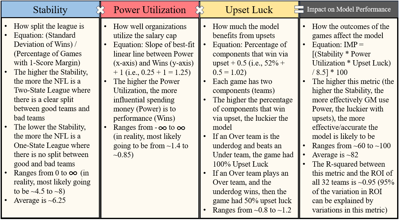
Measuring the Impact on the Model’s Performance
I have translated the elements of unpredictability that I believe most closely affect the model’s performance into three variables. The first is Stability, which describes how much the league is split into good and bad teams, or, in other words, how well the league is split into organizations in State 2 (pulling down/tanking) and State 4 (pushing up/going all in). In general, the larger the split, then the clearer the cycles, and therefore the more predictable the league is. The second is Power Utilization, which measures the impact that using Power has on the performance on the teams. The more impactful that spending money is, then the more predictable the league is. In other words, if teams spending a high level of their respective salary cap on their active roster win more games, and teams spending a lower level of their respective salary cap on their active roster win fewer games, then the more predictable the league is. The third is Upset Luck, which is the percentage of upsets that benefit the model. The easiest way to understand this one is to start with the idea that each game has two components (teams). The higher the percentage of components that progresses the bets towards winning via upset, the luckier the model. If an Over team (a team that I have predicted would win more games than the line from the sportsbook) is the Underdog (the team that the sportsbook believes will lose) and beats an Under team (a team that I have predicted would win fewer games than the line from the sportsbook) as the Favorite (the team that the sportsbook believes will win), then the game had 100% Upset luck, because both of the components progress the bets of both teams towards winning. If an Over team plays an Over team and the Underdog wins, then the game had 50% Upset luck no matter who wins.
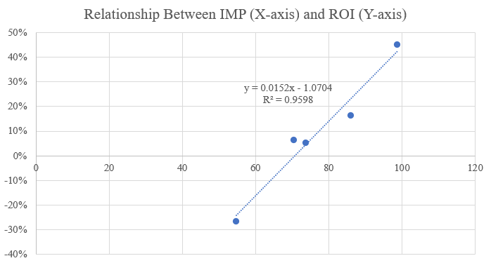
By combining these three elements together, I was able to create a singular variable that can be used to illustrate the unpredictability of the league, and if I am right about the cycles being accurate to expectations, then this Impact to Model Performance metric should be significantly correlated to the gambling performance of the model (here, the Return On Investment). With an R-squared (explained later) of ~0.96 (through the first 5 seasons), the gambling performance of this model is significantly impacted by the combination of these three variables, or, in other words, the predictability of the league.
Below is a chart illustrating the breakdown of Impact to Model Performance into its individual elements followed by an in-depth section on each one.
–
Stability
Circling back to the wavelength graph above and the metaphor of jumping, the ultimate goal of every NFL organization is to win the Super Bowl, and in order to do so, it should maximize its Crest. If the structure of the league causes the performance of these organizations to be cyclical, then the efficient way to maximize the Crest is to maximize the Amplitude by maximizing (the absolute value of) the Trough. Furthermore, if NFL organizations were to follow the natural rhythm of the waveform, then every team would be at or moving toward Phase 2 (pulling/tanking) or Phase 4 (pushing/going all in). There is little incentive for an organization to win 7-10 games (without making the playoffs), as it is not giving itself a chance to make a postseason run while also giving up valuable draft positioning and creating a harder schedule for itself in the following season. If an organization tries to compete every season, then they are risking becoming stagnant around the equilibrium, unable to break into the championship window in both the short- and long-term. Essentially, if the organization is going to perform poorly then it should perform as poorly as possible, and if it is going to perform well then it should perform as well as possible. This dichotomy is similar to a toggle mechanism like a light switch, where every NFL organization should either be “on” (Phase 4) or “off” (Phase 2). In terms of predictability, when someone flips a light switch, that person is not concerned whether or not it will flip back without some type of external stimulus. However, if that person tries to balance the lights switch between “on” and “off,” it’s much harder to predict whether the light will be on or off at the end. Zooming out to look at the league at a macro-level, every organization should hypothetically be in one of these two states (or at least close to reaching it). The closer that the organizations are to operating at one of these two states, the more stable the league is overall. Hypothetically, every Phase 4 organization would beat every Phase 2 organization that they played. The more stable the league is, the more predictable the league is. When it comes to gambling, the more predictable the event, the more financially attractive the bet is (ignoring odds).
The formula for “Stability” is:
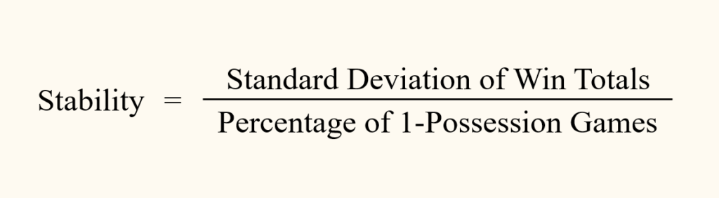
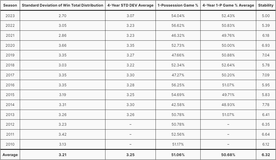
This metric combines two different types of predictability. The Standard Deviation of Win Totals measures the predictability at the season-level, and Percentage of One-Possession Games measures the predictability at the game-level. The more spread out the Win Total distribution is (meaning that the league is more split into one group of good teams and another group of bad teams), the larger the Standard Deviation. The more games where the scores of the two teams are separated by 8 or fewer points (the teams are more evenly balanced in terms of performance), the higher the Percentage of One-Possession Games. The scale for Stability is roughly 0 to 10, where 0 would the least stable, the “messiest,” or, in other words, the most competitively balanced the league could be. The purpose of the regular season in any sport is to effectively sort the teams of the league from the highest performing to the lowest. So if the league is “messy,” then the sorting has not been effective in separating the teams. An accurate sort is typically preferred as the result often determines seeding for the postseason. If every team went 8-8-1, then the Standard Deviation would 0. If not a single of the 272 games (currently as of 2025 – 17-game regular season) had a score differential of 8 or fewer points, the Percentage would be 0. There is a very low chance of either of those phenomena ever happening. An example of a Stability of 10 would be a Standard Deviation of 4 and 40% of the games being one-possession. While there could hypothetically be a Stability higher than 10, it is unlikely. From 2010-2023, the highest Standard Deviation was 3.66 (2020) with the average being 3.21, and the lowest One-Possession Game Percentage was 42.58% (2014) with the average being 51.06%. Therefore, in that 14-year period, the maximum possible Stability was 8.60, while the average was 6.29.
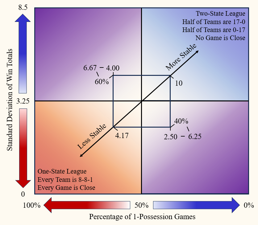
However, Stability will most likely lie within the smaller square in the graph above (around 4 to 7).
However, Stability will most likely lie within the smaller square in the graph above (around 4 to 7).
However, Stability will most likely lie within the smaller square in the graph above (around 4 to 7).
Looking at the graph above, the NFL falls somewhere in between the Two-State League and One-State League. The more it is like the One-State League, the harder it is to tell which teams are good or not. The more it is like the Two-State League, the easier it is to tell which teams are good or not. Understanding the cyclical nature of the league, it should have a Stability that leans more towards the Two-State League as organizations should either be pushing to go all in or pulling back to tank. However, football is never that clean, as injuries and upsets create instability, blurring the line between which teams are good and which ones are not.
So are this Stability metric and the performance of the model correlated? Using the Return on Investment of all 32 Win Total Futures bets each season as a representation for the performance of the model, the relationship had an R-Squared of 0.9127 from 2020-2023. Investopedia defines “R-Squared” as “a statistical measure that represents the proportion of the variance for a dependent variable that’s explained by an independent variable in a regression model.” The range of R-Squared is 0 to 1, where 0 means that none of the variance is a result of the independent variable, and 1 means that the variance in the dependent variable is entirely the result of the independent variable. In relation to this project, the independent variable is the Stability and the dependent variable is the Return on Investment generated by the model (using all 32 organizations via the Win Total Futures method). A high proportion of the variance in the Return on Investment is explained by the Stability metric. In other words, the Stability is largely responsible for the changes in the performance of the model. While the sample size is small, as there have only been 4 seasons of predictions, an R-Squared of over 0.9 would indicate a strong correlation. However, the correlation dropped significantly due to the 2024 season. An R-Squared of 0.69 would still indicate some level of correlation, but it’s clear that Power Utilization and Upset Luck also influence the ROI.


Personally, while I am certainly biased, I believe that the R-squared could have been even higher through the 1st four seasons. Close losses happen every season, but in 2023, there were multiple bets lost due to extremely unlikely outcomes. The Philadelphia Eagles, Kansas City Chiefs, and Jacksonville Jaguars all had Over bets placed on them, those bets all lost by 1 win, and each team had embarrassing upsets that prevented the bets placed upon them from being successful. A more in-depth analysis of the 2023 season can be found below. While I would not necessarily expect all 3 bets to flip from losing to winning, just one of the bets flipping to successful would have put the overall Return on Investment much closer to the best fit line on the graph above, thereby lowering the R-squared.
I should note that I checked whether or not the individual elements of the Stability metric were correlated or not. Ideally, when generating a metric such as Stability, the individual elements should be unrelated, as that could create a covariance issue. Unlike with Stability and Return on Investment above, in this case, I would want the Standard Deviation of Win Totals and Percentage of One-Possession Games to have a low correlation. That is because I am not trying to predict the Standard Deviation of Win Total via the One-Possession Games percentage or vice versa. Instead, I want Stability to be affected by either a change in Standard Deviation or a change in Percentage. The graphs below show that the two variables that compose the Stability metric are unrelated.
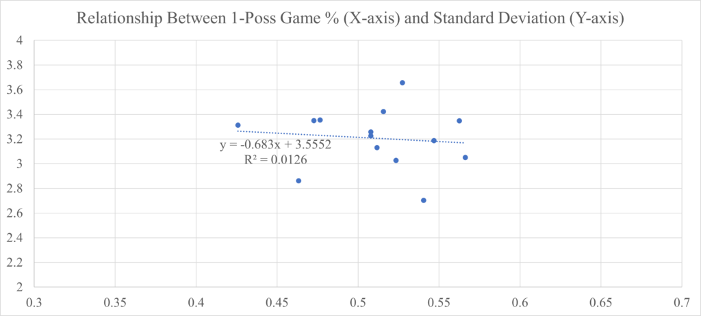
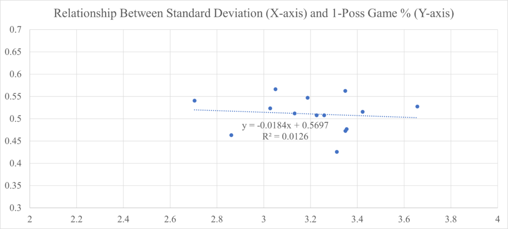
An R-Squared of 0.0126 would indicate that the variance in either variable is not explained by variance in the other variable. Or, in other words, they are unrelated. Because these two variables can be calculated for any season at any time (unlike Power Utilization and Upset Luck), I was able to go back further than the seasons for which I have predictions (2020) and further back than the seasons that currently comprise the model (2015). The two graphs above contain data going back to the 2010 season.
Let’s look at the trend of Stability for the league since 2010. In the period from 2010 to 2021, the Stability was relatively flat with an average of 6.5. If anything, there was a slight increase in Stability from season to season.
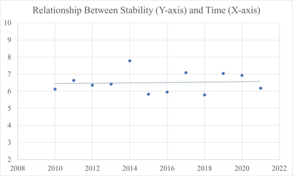
However, the 2022 and 2023 seasons changed the trend significantly.
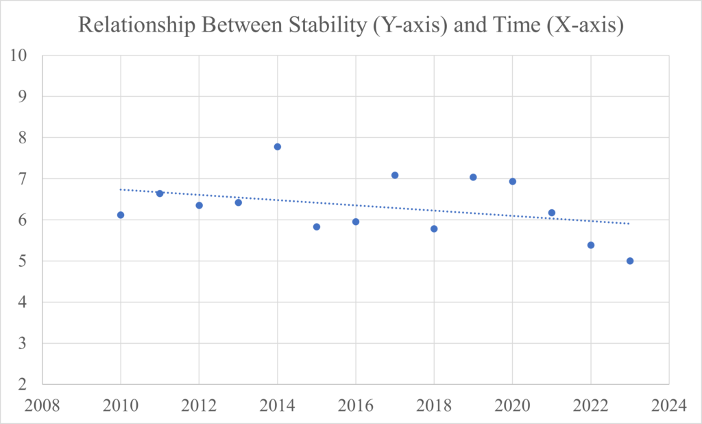
Both 2022 and 2023 had lower Stability than any other season since 2010, dropping the average for that period from 6.5 to 6.32. The potentially worrying aspect about this decline in Stability is that from 2020 to 2023, it was nearly linear. If this trend continues, this project and the structural integrity of the league could be in danger. As shown above, the predictability of the league is very influential to the success of the model. Why is the league becoming more unstable? Are there signs of the increase in unpredictability?
If you are a football fan, you probably did not need Tom Brady to tell you that the quality of the NFL has dropped over the last couple seasons (post-pandemic). I personally believe that the cause for the decline in quality is connected to the decrease in Stability. Two key impacts on the Win Total distribution and the Percentage of One-Possession Game are injuries and referee inconsistency. The quarterback is often considered the most important position on the field, and in 2023, there were a record-66 starting quarterbacks during the season. Whether it was due to injury or poor performance, a lack of consistency in quarterback play makes predictions more and more irrelevant. Quarterbacks are often a defining element of a team, so when two teams end up starting backup quarterbacks for whatever reason, the game will likely be more evenly balanced than if the starters were playing. While refereeing has always been controversial (especially in the NFL due to its insistence on limiting progression through technology or other means), the consistency in calls in the past couple seasons has been questionable at best. Whether its week-to-week or even quarter-to-quarter, what was a Holding penalty for one referee on one play might not be a Holding penalty for another referee on another play, even when most would say that the infraction was clearer on the latter play. While the NFL likes to joke that it is scripted in order to eschew any claims of referee foul play, it is undeniable that referees have the power to decide which team can have a sometimes game-winning advantage. Whether it’s how a referee crew botched the end of the 2023 Chiefs-Packers game or how just one referee helped determine the NFC playoff seeding through a careless assumption at the end of the Cowboys-Lions game. Both of these elements have pushed the Standard Deviation of Win Totals down and the Percentage of One-Possession Games up.
Does the NFL control how chaotic the league is? Would they want to push the Stability down? While quarterback injuries are probably not high on the list of objectives, the referees’ influence seems to make games closer than before, and the viewership data would suggest that it worked. While the NFL has other ways of generating revenue, a massive source is the TV rights to broadcast the games nationally. The 2023 season was one of the most viewed seasons in decades. CBS had its highest viewer average since returning to broadcasting NFL games in 1998. FOX, despite declining viewership across the network overall, posted its second-best NFL season since 2019 (only outdone by the 2022 season). NBC, home to Sunday Night Football, had its highest viewership since 2019. Monday Night Football, across ABC/ESPN/ESPN2, had its largest average audience since 2000. While these numbers are certainly influenced by the historic “double strike” of both the WGA and SAG-AFTRA (Entertainment industry unions), which limited the amount of competitive original content on broadcast, it would appear as though the NFL has significantly benefited by the recent decline in Stability.
In the end, the NFL regular season, like the regular season for any team-based sports league in the world, is a sorting algorithm. It’s purpose is to sort the teams within the league based on their abilities. Depending on the league, each team plays a certain number of games in order to determine which teams are better than the others. Of the Big 4 Sports in the United States (NFL, NBA, NHL, MLB), the NFL plays the fewest games by far (17, compared to 82, 82, 162, respectively). Therefore, every game matters immensely in terms of sorting the teams. If the sorting algorithm were 100% “accurate,” then the “better team” would beat every “worse team.” However, in reality, who is to say who the better team is? In a way, the sportsbooks do, but the existence of upsets would indicate that they do not always know either. This project attempts to do so, but in no way would everyone agree with the predictions from this model. But, as a reminder, the less stable the league is, the lower the standard deviation. The less stable the league, the more teams that are neither good nor bad. If the goal of the NFL is to indeed accurately sort the teams in order to award the best teams a spot in the postseason, then the league should want the sorting algorithm to be as accurate as possible, and, therefore, they should want a higher Stability. In sports, there are always going to be upsets, but if there are too many upsets (or if the upsets are too improbable), then the Stability, and therefore structural integrity, of the league can become compromised.
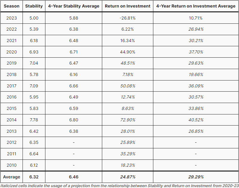
If the NFL does indeed not have an influence on the Stability, then a return to the long-term mean of 6.5 would be beneficial to the project. If one takes the linear relationship between Stability and Return on Investments from 2020-2023 and projects backwards in time across previous seasons, then the average performance of the model improves drastically. The table below helps illustrate this point.
–
What Happened in 2023?
If it felt as though that there were no dominant teams in 2023, it’s because there really weren’t any. The top teams in both the NFC and AFC had questionable losses, with the Ravens getting swept by the Steelers and a home loss to the Colts and the 49ers having a three-game losing streak against beatable teams. And there weren’t many bad teams either, other than the Panthers, who they themselves beat a Texans team that would end up making the Divisional round of the playoffs. The 4-13 Cardinals beat the 12-5 Cowboys, the 10-7 Steelers, and the 11-6 Eagles. The 4-13 Patriots beat the 11-6 Bills and the 10-7 Steelers. The 11-6 Browns started 5 different quarterbacks during the regular season, and every single one won at least 1 game. According to LastWordOnSports, the Browns were the first team in 35 years to start 4 quarterbacks and have a record above 0.500 through Week 14. Data science would say that these two seasons, 2022 and especially 2023, were outliers, and that Stability should regress back to the mean of 6.5. This unpredictability has led to more exciting finishes to games and a more exciting playoff race, as more games came down the final possession and teams were closer to a 0.500 record. However, I would say that this excitement was artificial, as it was not produced by high-quality football, but rather an (arguably forced) increase in completive balance that creates a better highlight on social media via a game-winning play than a compelling full rewatch of the game.
As shown in the table above, the 2023 season was by far the worst season in terms of performance of the model. If the model is predicting predictability, then 2023 was the least predictable season since at least 2010. While there were a high number of games that hung in the balance, there were actually 3 seasons in that time span that had a higher percentage of games with a point differential of 8 or fewer points.
So while the One-Possession Game Percentage in 2023 was certainly higher than average, it was really the distribution of Win Totals that brought the Stability to a new low. That means that the parity of the league had not been stronger since at least 2010. In my opinion, this parity was due to teams who were “on schedule” to perform poorly (according to the model) outperforming expectations and teams who should have been outperforming other teams underperforming (once again, according to the model). For example, three organizations spending less than 70% of their total salary cap on their respective active rosters made the playoffs (Green Bay Packers – 69, Tampa Bay Buccaneers – 67, Los Angeles Rams – 60). That level of spending was no mistake either. All 3 of those teams were exiting a championship window (in terms of the Buccaneers and Rams, literally as both won a Super Bowl, but the Packers got rid of their All-Pro QB and All-Pro WR). While these teams were in varying Head Coach and Quarterback situations, they all outplayed many of their opponents despite having a lower Power. The Packers had the youngest offense in the league and a Quarterback in his 1st year as the starter. After the season, each of the other NFC South teams made significant coaching changes (and maybe a couple of more should have happened) as a result of the Buccaneers outperforming all of them. The Rams swept the Seahawks, who spent 90% of their total salary cap in 2023, on their way to the 6th Seed in the NFC playoffs. The Seahawks fired their long-time (and potentially Hall of Fame-worthy) Head Coach (who also had influence over the roster) after they missed the playoffs by one game.
What’s interesting is that the Standard Deviation was not actually that low until the end of the season. In fact, the Standard Deviation of the on-pace Win Totals after Week 12 was 3.21. So two-thirds of the way into the season, the Standard Deviation actually matched the 10-year average.
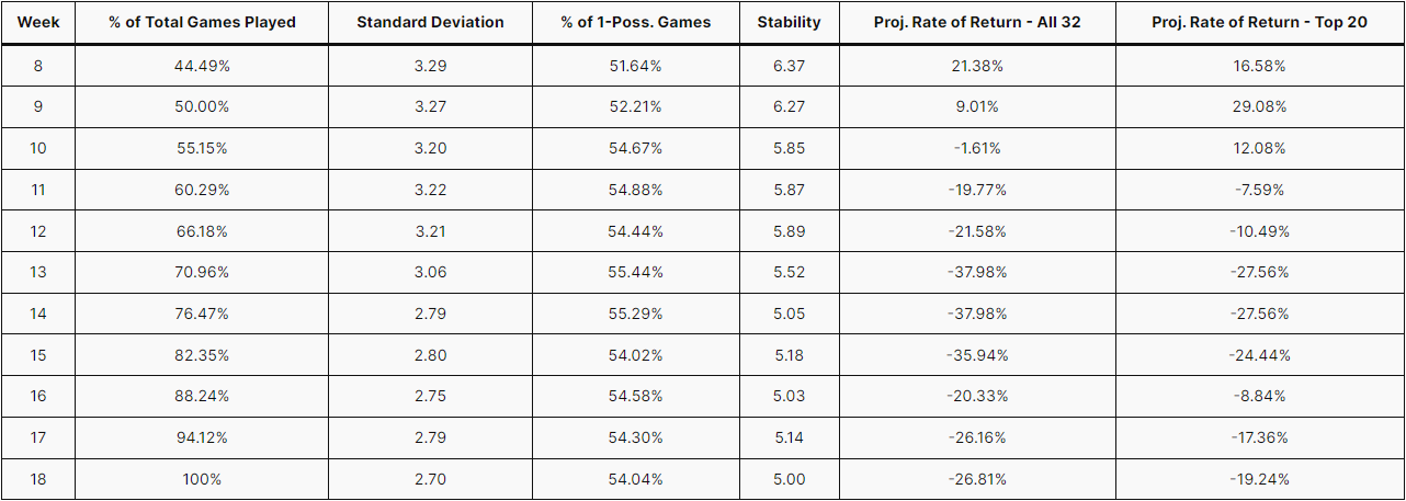
When looking at the relationship between Stability and projected Return on Investment at the week-by-week level, they are not as connected when compared to the season-to-season level. Regardless, the decrease in Return on Investment appears to occur roughly at the same times as the decreases in Stability. Part of the looseness of this connection is due to the nature of betting. There is no reward for being almost correct or more correct than needed (as in, winning a bet by more than one unit of measurement depending on the bet). Instead of being incremental, the payoff is binary, and here, that means that the changes in Return on Investment can be large and not necessarily dependent on the changes in Stability for a certain week.
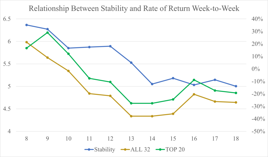
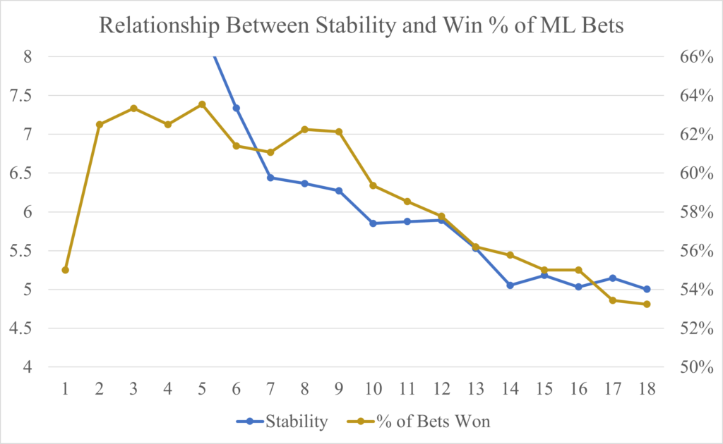
The chart below tells a similar story, but instead of the projected Return on Investment week-by-week, the Stability is being shown with the Percentage of correct Moneyline bets. For any given week, correct Moneyline bets are the total number of Over teams who won and Under teams who lost. Dividing the number of correct Moneyline bets by the total number of games played will generate the Win Percentage of Moneyline bets. This metric is a way to test how the model is performing in a way other than the projected ROI for Win Total Futures, which, as mentioned above, can be volatile. A general rule (although it may not be exact every single week), is that if the win percentage of Moneyline bets is high, then the ROI for Win Total Futures bets will likely also be high, and as a result, the model is performing well (and the league is likely more predictable than not). Starting in Week 7, there began to be large enough of a sample size of games to have a more realistic estimation of the Stability, and for Week 7-9, the model was looking like it would produce a high ROI for the Win Total Futures and a high Moneyline Win Percentage. The average Stability since 2010, excluding 2023, was 6.42, so there was no reason to believe that the Stability would not remain in the range that it was for those three weeks. However, Week 10 began the long and painful path toward a poor season in both ROI and Stability. A frankly overly-detailed analysis of the teams responsible can be found here.
–
Power Utilization
Simply put, if the league were predictable, then the organizations that spend more of their salary cap towards their active roster (as opposed to towards dead money) would win more games, and organizations that spend less would win fewer games. More spending should mean more talented players and therefore an elevated performance on the field. However, that is not always the case. Below is a graph showing how Power (percentage of the salary cap spent on the active roster) and Wins were related for the first 4 seasons (2020-2023).
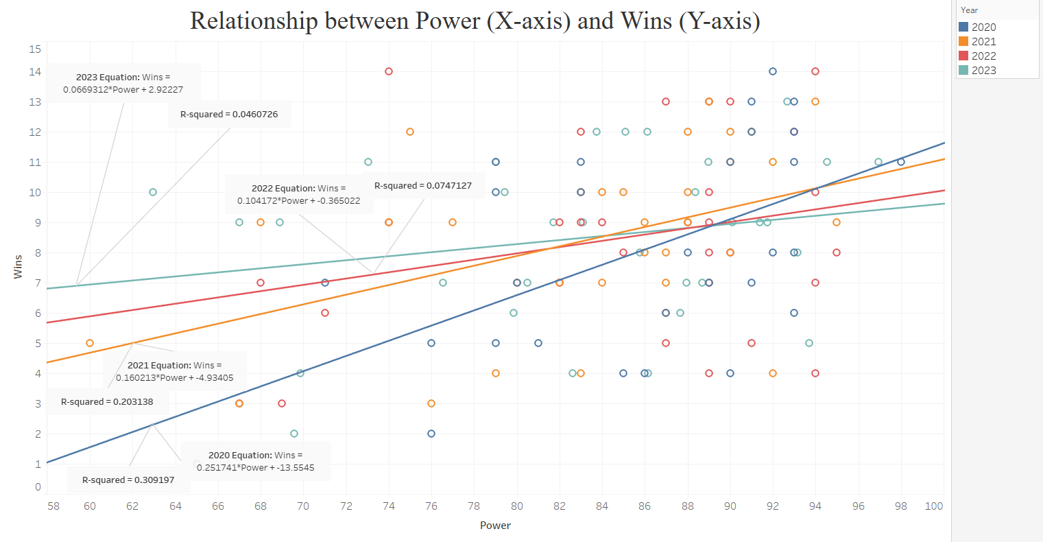
As one can see, the linear best fit line has been getting flatter every season since 2020, meaning that Power has been increasingly less positively related to Wins. Not only that, but the R-squared of the best fit lines steadily decreased every season, meaning that changes in Wins could explained by a smaller and smaller percentage of changes in Power. Basically, organizations that are spending a lot of money on their active roster are not consistently performing better on the field than organizations that are not. It’s more difficult to predict what should happen when that is the case. The next hurdle was to incorporate this relationship into the Impact on Model Performance metric, as the best fit lines have two numbers, the slope and the intercept. Fortunately, because the total number of Wins is typically the same every season (obviously there was a shift to 17 games in 2021, and Ties eliminate Wins, but the effect of both are negligible) and the average Power is typically always around 82, the slope is directly related to the intercept. In other words, they are equivalent, so I can just use one of them. Below is a chart that illustrates this connection.
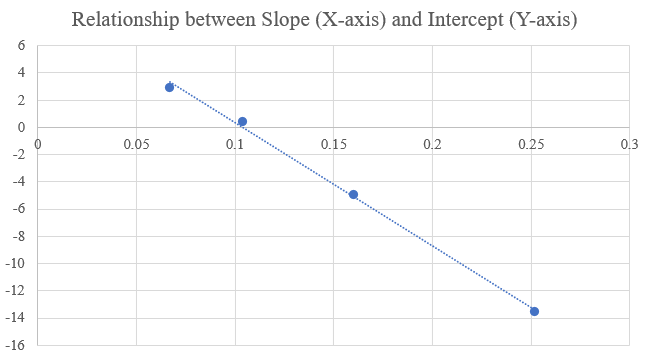
Since it did not really matter which one I picked, I decided to go with Slope to see if it relates to the Return on Investment, because that metric is more intuitive than the intercept. The more positively related Power Utilization is to Wins, the more positive the Slope. However, as one can see from the graph at the beginning of this section, the more positively related Power Utilization is to Wins, the more negative the Intercept, which could cause confusion. Having picked the Slope, is it related to Return on Investment? Similarly to the relationship between Stability and ROI, through the first 4 seasons, the R-Ssuared was above 0.9, indicating that the Power Utilization is significantly correlated to Return on Investment. That is intuitive, because the more influence spending money has, the more cyclical and predictable the league is, and therefore, the ROI should be higher. However, like with Stability, the R-squared dropped significantly in 2024, from 0.92 to 0.52. I would expect it to increase with additional seasons. It is important to remember that while each individual component should be somewhat related to the ROI of the model, the combination of Stability, Power Utilization, and Upset Luck should be even more so.


For the actual incorporation of the this metric into IMP, I wanted to alter the Power Utilization values so that it would never be negative, as that would become a problem for the IMP equation overall. In order to avoid those problems, I added 1 to the Slope.
–
What Happened in 2024?
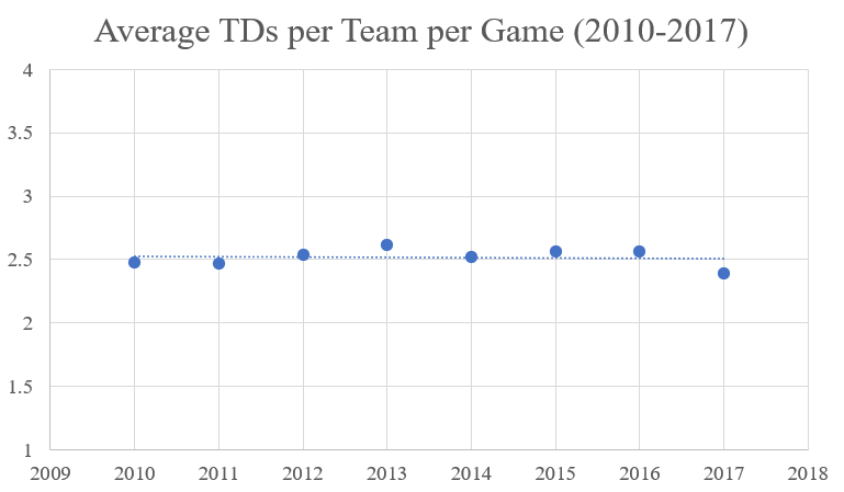
The Power Utilization was so low in 2024 that it was actually negative, meaning that the percentage of salary cap spent on the active rosters by each team was negatively related to the number of Wins for the respective teams. The more of the salary cap that organizations spent on their active roster, the worse they performed. But that should not have been entirely surprising. If one looks at the final graph in the Power Utilization section, it has steadily decreased since 2020. What is causing this trend? I would say that it is not solely one thing. It could be that Front Offices are simply just getting worse, but that would be a bit broad of a statement. Regardless, GMs are not spending money efficiently, but I think it is at least a little more complicated than that. Zooming out, it’s important to remember that the league is always changing. How teams are built and how they play are always in flux, shifting back and forth from pass-heavy to run-heavy and offense-focused to defense-focused. Specifically, there have recently (as of 2024) been some large shifts at the league level. Just looking at the period from 2010 to 2023, one can see a shift in offense. From 2010 to 2017, the average touchdowns scored per team per game was flat at around 2.5.
But from 2018 to 2021, offenses became the focus, increasing the average touchdowns per team per game from 2.5 to 2.7. That might not seem like much of a jump, but that increase is actually substantial, as that difference is across a league with 32 teams playing 16/17 games per season. I would think that this shift is due to the influx of new, more mobile quarterbacks, such as Patrick Mahomes (drafted 2017) and Lamar Jackson (drafted 2018), being combined with the older, stalwart quarterbacks like Tom Brady and Drew Brees still in the league before they retired. I would think that it would have been very difficult to build a singular defense that could compete against the entire spectrum of quarterback style (mobile, dual threat, pocket passer) in a single season.
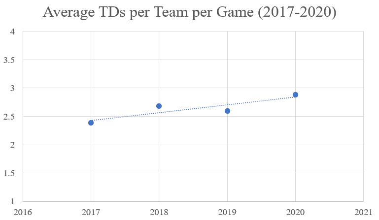
However, the average touchdowns per team per game returned to the long term average of around 2.5 from 2021-2023, which would indicate that offenses cooled down. A large part of that change is due to the older quarterbacks playing the more traditional style of the position retiring. Drew Brees retired after the 2020 season. Ben Roethlisberger retired after the 2021 season. Tom Brady retired after the 2022 season. The league had continued to shift towards quarterbacks who play more of a dual-threat type. As counter-intuitive as this statement sounds, this shift has allowed defense to more routinely prepare for one style of quarterback. In fact, towards the beginning of the 2024 season, there were legitimate analyst actually going on TV to suggest that Cover 2 (a less aggressive, more pass-oriented defensive formation with two deep safeties) should be banned. The formation was so effectively stopping this type of quarterback, because it makes throwing the ball harder, and these dual-threat quarterbacks were struggling to move the ball with their arms and not their legs.
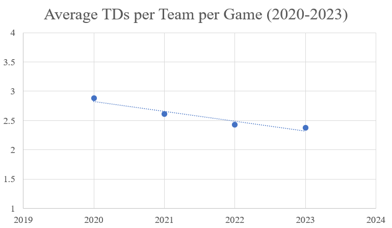
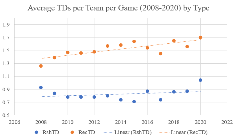
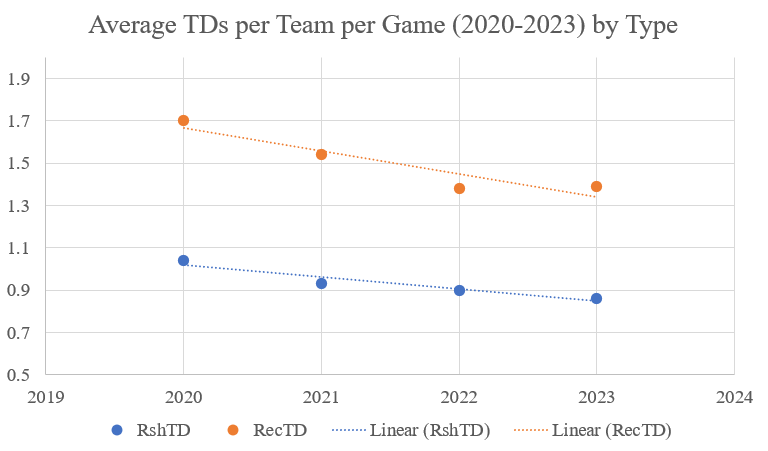
One can see this issue more clearly when the average touchdowns per team per game graphs are split by passing and rushing touchdowns. Outside of 2020, passing touchdowns were largely responsible for both the rise in average touchdowns per team per game and the decline.
All of that is to say that being a GM is not easy or simple, as accurately spending to win games is harder than it looks. However, unfortunately for this project, it is important in terms of the predictability of the league. Similarly to Stability’s correlation to ROI, Power Utilization had an R-squared of over 0.90 through the first four seasons. Also similarly to Stability, Power Utilization steadily decreased over the first four seasons of this project, supporting the idea that the league had become less stable over that period. I should note that Stability and Power Utilization are not automatically intertwined, as shown by 2024’s high Stability and low Power Utilization.

–
Upset Luck
This piece of the Impact on the Model’s Performance is less directly related to the predictability of the league than Stability and Power Utilization. While those metrics have to do with the results of the games in relation to the league and the spending of the individual Front Offices, this metric has to do with the results of the games in relation to the model’s predictions. In the most predictable league, the team that is designated by the sportsbooks as the Favorite would always be the winner. And then ideally for this project, every Over team would be the Favorite and every Under team the Underdog. However, that would be basically impossible, but thankfully that does not have to happen in order for this model to be successful. I should note that this element of IMP does not directly have to do with the total number of upsets, but rather how the upsets impact the model. Pretty much every season has between a 30-33% upset rate, so fluctuations in that metric are minimal.
The easiest way to explain Upset Luck is to start with the idea of components. Each game has two components, which are the two teams playing in a game (using the term “team” would get confusing later on with regards to referring to the team in one game versus the whole season). Because there are 32 teams and currently 17 games per team, there are 544 total components. A component benefits the model if the team is an Over and wins the game or if it’s an Under and loses the game. Component Win Percentage is the number of components that benefited the model divided by the number of total components. Another way of looking at this metric is to consider it the overall win percentage of the model at the game-level.

A 55% Component Win Percentage over the first four season means that for any given week with all 32 teams playing, 17 to 18 components were positive (an Over team wins or an Under team loses) and 14 to 15 components were negative (an Over team loses or an Under team wins). When there is an upset, there are variety of outcomes depending on the specific components in the game, which are displayed in the chart below.

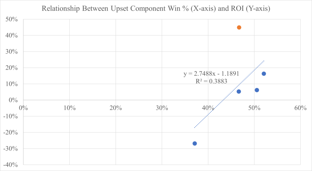
Upset Luck = (Upset Component Win Percentage across all 32 bets) + 0.5.
Upset Component Win Percentage is aggregated across the whole season with the average theoretically being around 50%. While I would hope that the non-upset games would have a higher Component Win Percentage than 50%, the upsets are much more random. In fact, I would think that if the model were predicting a stable and predictable league, then the Upset Component Win Percentage would be lower than 50%, as Over teams should not be the Underdog against Under teams as often as Under teams are Underdogs against Over teams. And through the first four season, this statement held true with the average Upset Component Win Percentage being 46.6% (as the average Stability in that time period is also lower than the long-term average).
One way to observe the impact of upsets is to look at the season if the Favorites won every game. Below is the Favorites Only version of the 2024 season.

This chart looks is very similar to the actual 2024 Win Total Futures chart. However, the main difference, other than it showing all of the results of the 2024 if every Favorite won, is the addition of two colors: orange and light green. If a team has either a red or dark green cell, then the Favorite won the actual game. If a team has an orange cell, then the team was involved in an upset, and the result for that team matches the model’s prediction (Over or Under the line). For example, the Steelers were the Underdog in Week 1, and they won, which matches the Win Total prediction of Over 8.5. That cell is therefore orange and filled with a 0 as they were supposed to lose. An orange cell will have a 1 if the team is an Under team, the Favorite, and the loser, such as the Bengals in Week 1. They were 8.5-point favorites over the Patriots and lost, which benefited the model. On the other hand, if a team has light green cell, then the team was involved in a upset, and the result does not benefit the model. The Falcons were an Over team, the Favorites in their Week 1 matchup against the Steelers, and lost the game, so the cell is light green and has a 1. The Patriots, an Under team, also have a light green cell in Week 1, but they were the Underdogs when they beat the Bengals, so there is a 0 instead.
While the orange is purposefully similar to red and the lime green to dark green, it is opposite in terms of the real effect on the bet. One example of an orange cell is an Over team that “should” have lost as the Underdogs, but in real life they won, so it actually had a positive effect on the model. Similarly, light green means that a positive result for the model should have happened, but in reality, the negative result for the model happened. The orange cells represent the model being “lucky,” and the light green cells represent the model being “unlucky.” The formula for Upset Luck can also be described as Upset Luck = [(# of orange cells / # of orange and light green cells) + 0.5].
The 2024 Steelers were involved in 8 upsets, winning 5 and losing 3, so their Favorites Only Win Total was 8, 2 less than the actual Win Total of 10. That number of Wins was still enough for the bet to win, as the line of 7.5 was lower than both 10 and 8. However, not all of the bets work out that way. For example, the Under bet on the 2024 Seahawks would have won if the Favorites had won in all of their matchups. Instead, the bet actually lost by multiple games. This difference can be seen in the chart above by the fact that they had 5 light green cells and only 1 orange cell.
Looking at the graph below, Upset Luck is much less correlated to the ROI of the model than Stability and Power Utilization. This lower correlation is due to the fact that an Win Total Futures bet can be successful despite having an individual Upset Component Win Percentage below 50% and vice versa. However, if 2020 is an outlier, then the correlation is actually around the same level as the other two elements of IMP through the first 4 seasons of the project (as shown in the first graph of the “What Happened in 2020?” section).
–
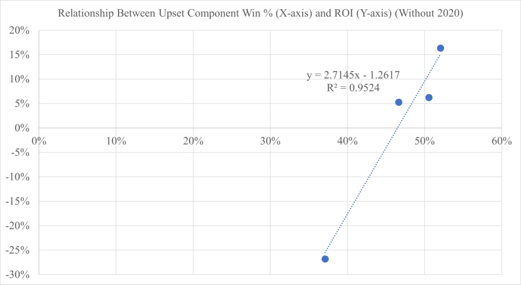
What Happened in 2020?
Compared to the graph directly above, the R-squared of the graph below is much higher, as it excludes the 2020 season. Despite having a similar Upset Luck (~0.96) as the 2024 season, the 2020 season had a far higher ROI (45% vs 5%), falling far out of the range of the graph below. How did this result happen when the other 4 seasons fit rather closely to the best fit line?
Another way to assess the “luckiness” of the model is to compare the number of bets that would have flipped either way (win to loss and loss to win) if only the Favorites won every game. Below is a chart that shows the flips in both directions for every season from 2020 to 2024. With a total “flipped record” of 20-19, the model has been pretty much even in terms of “luckiness” through the first 5 seasons. I would expect this record to stay around 0.500 long-term.

However, there is a more specific way to access how upsets have affected the model. Instead of just looking at the number of flips, one could look at the difference in ROI between the Favorite Only version and the actual outcomes. If the actual ROI is higher than the Favorites Only ROI, then the model was lucky, and if the Favorites Only ROI is higher than the actual ROI, then the model was unlucky. Below is a chart that sums up the relationship between these two metrics over the first 5 seasons of the project.

Through the first 5 seasons, the model has been lucky in terms of Difference in ROI (+2.93%) but not in terms of % of Upsets that Benefit Model (46.60%). This discrepancy is due to the fact that total number of orange cells does not directly equate to any individual bet winning or losing. For example, in 2020, the total number of light green cells outnumbered the orange ones, but the Actual ROI was still higher than the Favorites Only ROI. This combination of circumstances is possible due to the fact that bets can win in reality despite having more light green cells than orange. The 2020 Buccaneers (Over 9) went 1-3 in upsets but still finished with 11 wins, which means that the bet still won. The Favorites Only version of the 2020 season is below.

While the 2020 season was “lucky” due to having a positive Difference in ROI between Actual and Favorites Only despite a % of Upsets that Benefit Model below 50%, the luckiest season was actually the 2021 season with a Difference in ROI of 37.74%. When looking at the Favorites Only version, 8 winning bets would have lost, and 1 losing bets would have flipped to winning. However, the 2023 season was just as unlucky as the 2021 season was lucky. 8 losing bets would have won in the Favorites Only version, while just 1 winning bet would have flipped to losing. Over 40% of ROI was lost to upsets that season. Overall, it would appear as though the 2021 and 2023 seasons were outliers. I wouldn’t want to make a very small sample even smaller, but let’s say we take out both of those seasons.

In this scenario, the model would overall be even luckier. Actual ROI would go from 9.19% to 18.80%, Favorites Only ROI from 7.43% to 12.17%, and Difference in ROI from 1.76% to 6.64%. In the long run, I would expect the actual ROI to stay around 7.5-15%, Favorites Only ROI 7.5-15%, Difference in ROI 0%, and Percentage of Upsets that Benefit Model (Upset Component Win Percentage) slightly below 50%.
–
Name Explanation
The name ego Analytics contains two separate meanings. The first is an acronym – e.g.o. – standing for evenly gifted organizations. This phrase refers to the idea that every NFL organization has a relatively even playing field, or at least once did. Each organization could have the same number of draft picks and limit of how much they could spend on players. However, as seasons go by, organizations sign and trade players and draft picks, leading to the unevenness between organizations. The key is that the unevenness in the NFL is due to the decisions of the organization, not aspects like the differences in financial resources between the owners or in values between home markets.
The second meaning of the project’s title is a reference to psychology. In colloquial usage, ego would be described as one sense of self. For example, someone having a large ego means that he or she thinks of themselves highly and has high self-esteem. Professional athletes are known for having notoriously huge egos, but that quality is not necessarily a negative. If these athletes are competing at the highest level possible, then they must believe themselves that they are truly the best. These athletes have dedicated their lives to being one of, if not the, best in the world at what they do. The mentality to be the best has to be ingrained in professional athletes from a young age. But this mentality, at least in the NFL, also extends to others who work in professional sports, including the Head Coach (HC) and the General Manager (GM) specifically. If there are only 32 possible job openings for each position in the NFL, then every aspiring HC or GM in the entire world is fighting for one of those spots. Like the players, the HCs and GMs have to constantly prove that they deserve to be in the NFL.
The GMs (and the Front Offices) are trying to handle assets (players) as efficiently as possible by either pushing (accumulating as many current high-quality assets as possible) or pulling back (accumulating as many future high-quality assets as possible). Depending on the specific organization and year, there could be two objectives for them: either win a Superbowl in the upper section of the cycle or not get fired during the lower section.
Players, on the other hand, are trying to maximize the financial value for their performances. Depending on the quality of the specific player, there is a spectrum of objectives for them with two ends. For the higher quality end, it is to convince an organization to pay you as much money as possible, and for the lower quality end, it is to convince an organization that you are worth having on the team at all.
The HCs (and the Coaching Staffs) are theoretically trying to use the assets that they are given by the GM as efficiently as possible, but they have a similar split to the GMs and players. The HCs with the best rosters are trying to win as many games as possible in the hope of getting a favorable playoff seed (average/poor performances with good rosters can get an HC fired), and the HCs with poor rosters are trying to lose as many games as possible in hopes of getting a favorable draft position (average/good performances with poor rosters can create problems with the GM).
Therein lies the organizational tension. The players want to get the upper hand on the GMs by getting paid more than their value, and GMs want to get the upper hand by getting the best deal out of the players. If high-quality players do not think that they are being used in a way that showcases their value (and therefore justifying their future financial compensation), then they can take their frustrations out on the HC. If the HC does not think that the high-quality players are not properly executing their game plan (and therefore not winning games) then they can take their frustrations out on the players. When an organization performs poorly, the owner (or whoever makes these decisions) must make a decision of whose fault it is: either the HC or the GM (in some cases both are fired). The GMs will take the position that the roster that they assembled is perfectly fine, and the HC was the one who was incapable of utilizing the assets properly to win games. HCs will take that position that they did as much as they could with what they were given, and the GM was the one who was incapable of acquiring the assets necessary to win games. While players are not necessarily “fired” by ownership, they can be traded or released if expectations are not met.
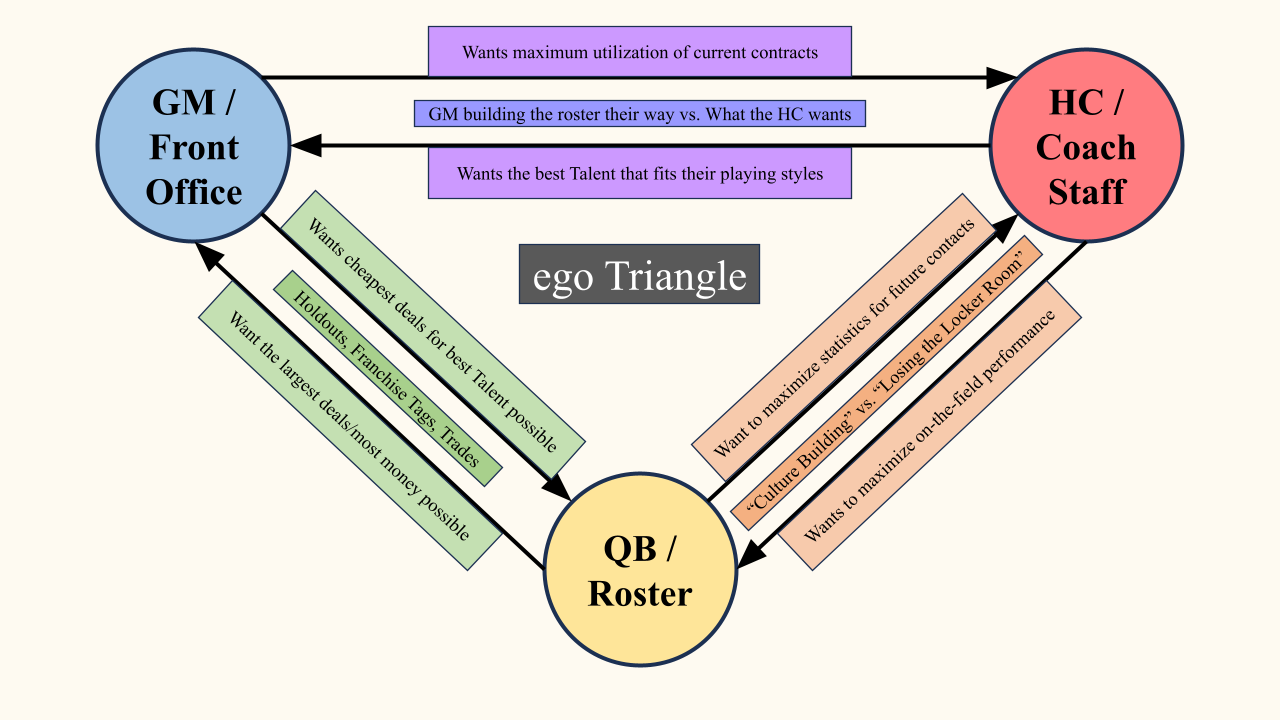
The triangular balance between these three entities creates a delicate and complicated microeconomic environment within the organization, especially given the downward pressures on performance caused by the cyclical nature in the NFL. The situation gets even more complicated when adding in the other 31 organizations who are all operating alongside (off the field) and against each other (on the field) in a larger macroeconomic environment. Understanding, tracking, and evaluating how each organization performs within these environments is one of the main objectives of this project.
In Freudian usage, ego is one of the three portions of the human personality, along with the id and the superego. According to Britannica, the ego is “experienced as the ‘self’ or ‘I’ and is in contact with the external world through perception. It is said to be the part that remembers, evaluates, plans, and in other ways is responsive to and acts in the surrounding physical and social world.” The id, on the other hand, is “the agency of primitive drives,” while superego is “the ethical component of personality.” Ego encompasses the executive functions which orchestrate the connection between the inner and outer worlds and the balance between the id and the superego. In the context of this project, the egos of the three groups mentioned above (GMs, HCs, and players) can help determine the health of the organization at both the micro- and macroenvironmental level. On the micro- level (within the organization), the interactions between the ids and superegos will create the balance of the objectives mentioned in the previous paragraph for each of the groups. A superego-led organization will have GMs, HCs, and players putting the organization first, above themselves. This organization-centric (superego-driven) culture can show its influence in various ways. A player could take a team-friendly deal, freeing up cap space to allow the GM to make the rest of the roster better. A GM could support the HC by accurately gathering and paying assets (players) that will be used effectively in the HC’s specific system (style). A HC could alter his system in order to maximize the value of the assets on the roster. A self-centric (id-driven) culture can show its influence in various ways as well. A player could refuse to practice or play (hold out), because they do not feel like they are not getting paid enough. A GM could splurge on high-profile, splashy players who do not really fit the HC’s system, and then throw the HC under the bus when the team does not perform well. A HC could let their personality clash with the players on the roster and refuse to alter their system, failing to maximize the value (strengths) of the assets (players).
It is unlikely that any person or organization is completely led by either the superego or the id, and that is where the ego plays a crucial role. While the examples above show one side of the two portions of the human conscience (superego in the positive and id in the negative), the inverse could be true, with selfish (in a literal sense) behavior leading to higher performance. As seen in several areas of society, acting unethically can provide benefits that acting ethically cannot. However, football is often considered the ultimate team-sport, so actions that are superego-driven (putting the team first) are often lauded and seen as reasons for success. The egos of GMs, HCs, and players will dictate the actions of each NFL organization, and understanding how those off-the-field actions impact the on-the-field results is another one of the cornerstones of this project.